Worked Example
Description
A study of the electronic structure and vibrational spectrum of 1,4-divinyl-benzene (at the B3LYP/STO-3G level of theory) using Gaussian03W.

Configuring GaussSum
I opened the Settings dialog box, by clicking on File/Settings, and verified that the location of the Gnuplot executable was correct by clicking on the Test button.
Geometry optimisation
- Input file: [PhCCCC_gopt.gjf]
- Partial output file: [PhCCCC_gopt_partial.out]
- Complete output file: [PhCCCC_gopt.out]
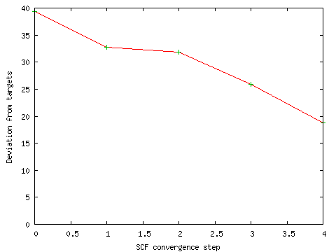
During the initial SCF calculation, I ran GaussSum ("Monitor SCF"; defaults; PhCCCC_gopt_partial.out) to see whether the calculation was converging. The result is shown below. The line is heading towards zero, which indicates that the SCF is converging.
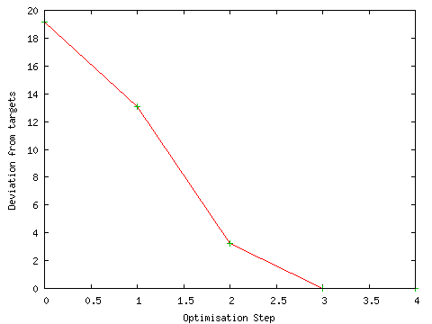
The progress of the geometry optimisation was also monitored during the calculation. The geometry optimisation proceeded smoothly to an energy minimum as shown by the graph below ("Monitor GeoOpt"; defaults; PhCCCC_gopt.out).
Molecular orbital information
- Input file: [PhCCCC_gopt.gjf]
- Output file: [PhCCCC_gopt.out]
- GaussSum outputs: [gausssum2.1/orbital_data.txt] [gausssum2.1/DOS_spectrum.txt]
I extracted the molecular orbital information from the output file of the geometry optimisation ("Orbitals"; defaults; PhCCCC_gopt.out). Molecular orbital information was written to the orbital_data.txt file in a subdirectory called gausssum2.1. Information on the frontier orbitals is shown below.
MO		eV	Symmetry
40	L+4	7.42	BG
39	L+3	4.96	AU
38	L+2	3.01	BG
37	L+1	2.46	AU
36	LUMO	1.02	AU
35	HOMO	-4.17	BG
34	H-1	-5.31	BG
33	H-2	-5.78	AU
32	H-3	-7.17	BG
31	H-4	-7.82	AG
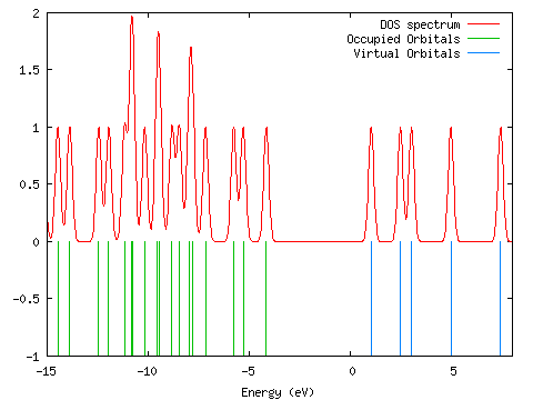
A density of states diagram was convoluted from the molecular orbital data ("Orbitals"; DOS, start=-15, end=8, FWHM=0.3; PhCCCC_gopt.out). It is shown below. The data used to draw this graph is contained in gausssum2.1/DOS_spectrum.txt.
- Input: [PhCCCC_pop.gjf]
- Output: [PhCCCC_pop.out]
- GaussSum input: [gausssum2.1/groups.txt]
- GaussSum outputs: [gausssum2.1/orbital_data.txt] [gausssum2.1/DOS_spectrum.txt] [gausssum2.1/origin_orbs.txt]
I wanted to describe each molecular orbital in terms of a percent contribution from the benzene portion, and a percent contribution from the divinyl portion. GaussSum can use Mulliken population analysis to do this (please be aware that Mulliken population analysis has some severe shortcomings). First of all, I needed to make Gaussian output orbital overlap information and information on the molecular orbital coefficients. This required a single point energy calculation with the keywords POP=FULL IOP(9/33=1,9/36=-1).
Next, I created a file called groups.txt in the gausssum2.1 subdirectory, which contained the following lines:
atoms
C6H4
1-8,19-20
C=C
9-18
Finally, I used GaussSum to calculate the molecular orbital contributions again ("Orbitals"; defaults; PhCCCC_pop.out, gausssum2.1/groups.txt). This time, orbital_data.txt contained more information (see below for information on the frontier orbitals). The HOMO is about 50/50 C6H4 and divinyl. The so-called 'accurate values' should be ignored, although they are required for the "Electronic transitions" option to calculate changes in electron density. (Note that these columns are tab-separated and so can be imported easily into spreadsheet software.)
MO		eV	Symmetry	C6H4	C=C	Accurate values (for the Electronic transitions module)
38	L+2	3.01	BG	17	83	0.168430209324	0.83157002452
37	L+1	2.46	AU	100	0	0.999818653049	0.000181859510613
36	LUMO	1.02	AU	54	46	0.543282127318	0.456725399153
35	HOMO	-4.17	BG	54	46	0.541778503997	0.458228594354
34	H-1	-5.31	BG	100	0	0.999877441172	0.000141570363359
33	H-2	-5.78	AU	15	85	0.154899304133	0.845103027118
The initial DOS spectrum created by GaussSum did not include any of the virtual orbitals. As a result, I wanted to change the start and end point of the spectrum, but I did not want to recalculate all of the contributions of the groups. I set "Use existing orbital_data.txt?" to TRUE, and altered the values of start and end until I was happy ("Orbitals"; start=-15, end=8, FWHM=0.3, "Use existing orbital_data.txt?"=TRUE; PhCCCC_pop.out):

A nicer image can be created using spreadsheet software, or a program such as Microcal Origin, and the file gausssum2.1/DOS_spectrum.txt. The image below was created using Microcal Origin (for Linux, try Scigraphica or Grace).

Instead of drawing a DOS curve, you may prefer to use a more straightforward depiction of the breakdown of molecular orbitals between various groups in a molecule. To do so, set "Create originorbs.txt" to TRUE, and rerun GaussSum ("Orbitals"; start=-15, end=8, FWHM=0.3, "Use existing orbital_data.txt?"=TRUE, "Create originorbs.txt?"=TRUE; PhCCCC_pop.out). Origin or Grace may then be used to create the image shown below using the data in gausssum2.1/origin_orbs.txt (it may take some practice - in Origin you need to set the columns XYXY, and plot the four columns using 2-point segments).

- Input: [PhCCCC_pop.gjf]
- Output: [PhCCCC_pop.out]
- GaussSum input: [gausssum2.1/groups.txt]
- GaussSum outputs: [gausssum2.1/COOP_data.txt] [gausssum2.1/COOP_spectrum.txt]
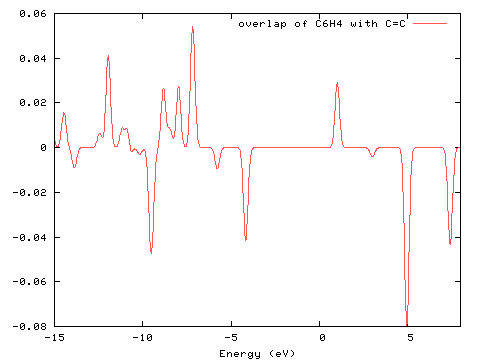
The interaction between the two groups can be visualised using a COOP (Crystal Orbital Overlap Population) diagram. This interaction is measured by the degree of positive/negative overlap for a particular molecular orbital. For more information on its use, see the paper of Herlem and Lakard listed in the bibliography. The diagram below was created from PhCCCC_pop.out using GaussSum ("Orbitals"; COOP, start=-15, end=8, FWHM=0.3; PhCCCC_pop.out, gausssum2.1/groups.txt).
Vibrational spectrum
- Input: [PhCCCC_IR.gjf]
- Output: [PhCCCC_IR.out]
- GaussSum outputs: [gausssum2.1/IRSpectrum.txt] [gausssum2.1/IRSpectrum.txt (after scaling)]
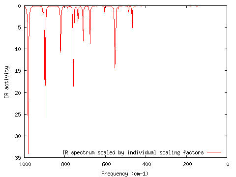
I calculated the vibrational frequencies of divinylbenzene and their associated IR intensities. GaussSum extracts this information from the log file into gausssum/IRSpectrum.txt ("Frequencies"; start=0, end=1000, num pts="500", FWHM=3, Scaling factors=(General,1.00); PhCCCC_IR.out):
Normal Modes
Mode	Label	Freq (cm-1)	IR act
1	AU	52.7881		0.0323
2	BG	83.9368		0.0
3	AU	148.1571	0.3826
4	BU	178.6727	0.2686
I wanted to scale all normal modes greater than 1000 cm-1 by 0.5 (this is not a real example! :-). I opened IRSpectrum.txt in Excel, and changed the values for the scaling factors from 1.00 to 0.5 for those normal modes greater than 1000 cm-1. I resaved IRSpectrum.txt in the same format (Tab-separated) and location. After choosing the "Frequencies" option I chose "Individual scaling factors" and ran GaussSum again ("Frequencies"; start=0, end=1000, num pts=500, FWHM=3, scaling factors=Individual; PhCCCC_IR.out, gausssum2.1/IRSpectrum.txt). The result is shown below.
UV-Visible Spectrum
- Input: [PhCCCC_TD.gjf]
- Output: [PhCCCC_TD.out]
- GaussSum outputs: [gausssum2.1/UVSpectrum.txt] [gausssum2.1/UVData.txt]
I wanted to calculate the UV-Vis absorption spectrum of divinylbenzene. I added the keyword IOP(9/40=2) to the TD-DFT command, to output information on smaller contributions to each electronic transition.
I ran the "Electronic transitions" option with the default settings ("Electronic transitions"; start=300, end=800, num pts=500, fwhm=3000; PhCCCC_TD.out) but no graph was drawn, and there was a message "There are no peaks in this wavelength range!". I looked at gausssum2.1/UVData.txt and saw that the lowest energy peak was at about 230nm. I ran the "Electronic transitions" option again, this time using more appropriate values for the start and end of the diagram ("Electronic transitions"; start=170, end=270, num pts=500, fwhm=3000; PhCCCC_TD.out) and the result is shown below (this information is written to gausssum2.1/UVSpectrum.txt).

The file gausssum2.1/UVData.txt is created containing the following information:
No.	eV      nm      Osc.Str.  Symmetry
1	5.3351	232.39	0.1695	Singlet-BU
2	5.3747	230.68	0.6789	Singlet-BU
3	6.2152	199.48	0.0	Singlet-AG
Because I ran the "Orbitals" module earlier using a groups.txt, information about the change in the electron density of various groups in the molecule is also printed in gausssum2.1/UVData.txt. Note that this information is very approximate, as it is calculated on the basis that the squares of the contributions of the various one-electron transitions equals one, which is *not* true, but may be almost true :-).
No.	Major contribs                           Minor contribs  C6H4           C=C
1	H-1->L (47%), H->L (-15%), H->L+1 (36%)                  76-->71 (-5)   24-->29 (5)
2	H-1->L (13%), H->L (61%)                 H->L+1 (6%)     62-->58 (-4)   38-->42 (4)
3	H-2->LUMO (62%), H->L+2 (-38%)                           30-->40 (10)   70-->60 (-10)